In a prior post, I discussed scenario analysis using the OFFSET function. Today I would like to introduce you to two useful formulas, the “Index” and “Match” functions, which can actually be combined to create an even more useful “super” formula if you will. This formula can be used in place of the commonly used HLOOKUP and VLOOKUP functions in financial modeling, and is most useful when looking at information related to things such as “comps” tables or sensitivity analysis.
MATCH
The MATCH function returns the relative position of an item in an array, or series of data, that matches a specified value, in a specified order. The syntax for the MATCH function is:
=Match(lookup_value,lookup_array,match_type)
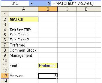
Below is an example of the MATCH formula in Excel. In this example, we have told the MATCH formula to search for the value in cell B11, “Preferred”, out of a range of choices that are captured in the data series found in cells A5 thru A9. We have also specified a match-type of “0” to indicate that we are interested in an exact match (1).
Remember – MATCH returns the position of the matched value within the look-up_array, and not the actual value itself. In the case below, MATCH has told us that “Preferred” can be found in the 3rd position (from the top) in the range selected.
INDEX
The INDEX function can be used to return an actual value found in a particular cell in a table or array by selecting a specific row and column in such table. The syntax for the INDEX function is:
=INDEX(array,row_num,column_num)
Think about playing the game Battleship. Array represents the landscape of the ocean and the row number and column number simply give us the coordinates.
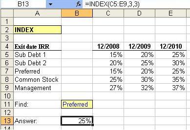
Below is an example of the INDEX formula in Excel. In this example, we have told the INDEX formula to search a table, defined by the area for columns C thru E and rows 5 thru 9. When searching the table, the formula will begin its search in the upper-left most cell in the table (cell C5 in this case), where the position would be defined as Row 1, Column 1. In our case, we are searching for the cell located at the intersection of the 3rd row and 3rd column in the table and want to return the value found in this cell. The location of the desired cell is E7 and you will notice that the formula in B13 has returned the correct value of 25%, found in E7!
A Perfect (INDEX) MATCH
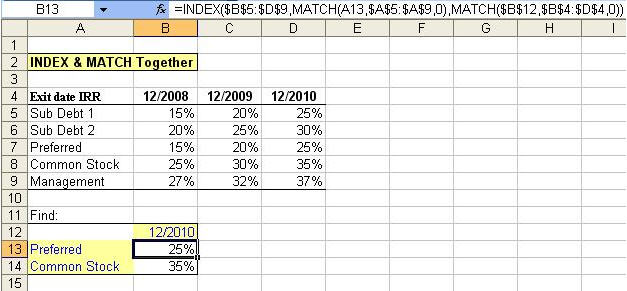
Now that we have seen both the MATCH and INDEX functions used separately, we are ready to combine the two formulas into one! Let’s take another look at the above table which is full of information regarding IRR’s for several different groups of investors and for several different investment exit years. Our INDEX formula in cell B13 seems to be limited by the fact that we have hard-coded exactly which row (3) and which column (3) we would like to select in order to return a value for the Preferred shareholders in the exit year 2010 (25%).
In order to make the INDEX formula more dynamic, below we are using the MATCH formula to help us tell the INDEX function which row and which column we would like it to choose. The second part of the INDEX formula is intended to tell the formula which row to select, and in place of the number “3” we have input “MATCH(A13,$A$5:$A$9,0).” If you recall how the MATCH formula works, it tells Excel to return the position of a designated value. In this case, our designated value is found in cell A13, “Preferred.” Our array for looking up “Preferred” is $A$5:$A$9, or the list of various investors. Because “Preferred” is located in the 3rd position in the array, the MATCH formula will provide a numerical result of “3”, telling the INDEX formula to select a value in the 3rd row of the INDEX array.
This same technique is used to tell the INDEX formula how to select its column number. Our final result is a returned value of 25%, the correct IRR for the Preferred investors in the exit year of 2010!
Getting Results:
Going forward, we can simply input a new year into cell B12 or a new class of investors into cell B13 to get our results. This is yet another example of how powerful a tool Excel can be, and we encourage you to read up on additional functionality concerning these two formulas by simply hitting “F1” in Excel to search for more information. Stay tuned for more useful modeling tips from Wall Street Prep!
(1) Match_type can be the number -1, 0, or 1 (default is 1), where “1” finds the largest value that is less than or equal to the look-up value (look-up_array must be placed in ascending order), “0” finds the first value that is exactly equal to the look-up value, and “-1” finds the smallest value that is greater than or equal to the look-up value (look-up_array must be placed in descending order).