- What is the Excel COUNTIFS Function?
- How to Use COUNTIFS Function in Excel?
- Excel COUNTIFS vs. COUNTIF: What is the Difference?
- Excel COUNTIFS Function Formula Syntax
- Text Strings and Numeric Criterion
- Date, Text and Blank and Non-Blank Conditions
- Wildcards in COUNTIFS
- COUNTIFS Function Calculator – Excel Model Template
- Excel COUNTIFS Function Calculation Example
What is the Excel COUNTIFS Function?
The COUNTIFS Function in Excel counts the total number of cells that meets multiple, rather than one, criteria.
How to Use COUNTIFS Function in Excel?
The Excel “COUNTIFS” function is used to count the number of cells in a selected range that meets multiple conditions as specified by the user.
Given set criteria, i.e. the set conditions that must be met, the COUNTIFS function in Excel counts the cells that fulfill those conditions.
For example, the user could be a professor looking to count the number of students that received an “A” score on a final exam, of the students that attended a review session held before the exam.
Excel COUNTIFS vs. COUNTIF: What is the Difference?
In Excel, the COUNTIFS function is an extension of the “COUNTIF” function.
- COUNTIF Function → While the COUNTIF function is useful for counting the number of cells that meet certain criteria, the user is constrained to only one condition.
- COUNTIFS Function → In contrast, the COUNTIFS function supports multiple conditions, thereby making it more practical due to its broadened scope.
Excel COUNTIFS Function Formula Syntax
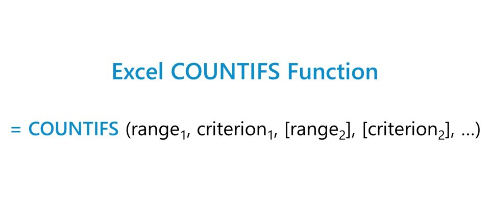
The formula for using the COUNTIFS function in Excel is as follows.
- “range” → The selected range of data that the function will count the cells within that match the stated criterion.
- “criterion” → The specific condition that must be met to be counted by the function.
After the initial two range and criterion inputs, the rest have brackets surrounding them, which are meant to denote that those are optional inputs and can be left blank, i.e. “omitted”.
Unique to the COUNTIFS function, the underlying logic is based on an “AND” criteria, meaning that all the conditions listed must be met for a cell to be “counted”.
Said differently, if a cell meets one condition, yet fails to meet the second condition, the cell will NOT be counted.
For those wanting to use the “OR” logic instead, multiple separate COUNTIFS functions can be used and then added together.
Text Strings and Numeric Criterion
The selected range can consist of text strings such as the name of a city (e.g. Dallas), as well as a number like the population of the city (e.g. 1,325,691).
The most commonly used examples of logical operators are the following:
| Logical Operator | Description |
|---|---|
| = |
|
| > |
|
| < |
|
| >= |
|
| <= |
|
| <> |
|
Date, Text and Blank and Non-Blank Conditions
In order for a logical operator to function properly, it is necessary to enclose the operator and criterion in double quotes, otherwise the formula will not work.
There are exceptions, however, such as a numeric criterion where the user is looking for a specific number (e.g. =20).
In addition, text strings containing binary conditions such as “True” or “False” are not required to be enclosed in parentheses.
| Criterion Type | Description |
|---|---|
| Text |
|
| Date |
|
| Blank Cells |
|
| Non-Blank Cells |
|
| Cell References |
|
Wildcards in COUNTIFS
Wildcards are a term that refers to special characters such as a question mark (?), asterisk (*), and tilde (~) in the criterion.
| Wildcard | Description |
|---|---|
| (?) |
|
| (*) |
|
| (~) |
|
COUNTIFS Function Calculator – Excel Model Template
We’ll now move on to a modeling exercise, which you can access by filling out the form below.
Excel COUNTIFS Function Calculation Example
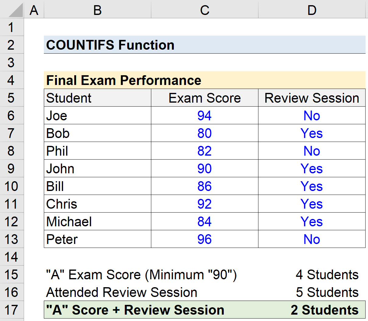
Suppose we’re given the following data on a classroom’s final exam performance.
Our task is to count the number of students that received a score of an “A” on a final exam, i.e. greater than or equal to a score of 90%, that also attended the review session prior to the exam date.
The left column contains the names of the students in the class, while the two columns to the right state the grade received by the student and the status of review session attendance (i.e. either “Yes” or “No”).
| Student | Final Exam Grade | Review Session Attendance |
|---|---|---|
| Joe | 94 | Yes |
| Bob | 80 | No |
| Phil | 82 | No |
| John | 90 | Yes |
| Bill | 86 | Yes |
| Chris | 92 | Yes |
| Michael | 84 | No |
| Peter | 96 | Yes |
Our goal here is to evaluate the effectiveness of the review session to see if there is a notable correlation between two factors:
- Review Session Attendance
- Earning a Minimum Grade of 90% (“A”)
With that said, we’ll begin by counting the number of students that earned an “A”, followed by the number of students that attended the review session.
The COUNTIF function can be used to calculate each figure, since there is only one condition each.
Of the ten students in the class, we’ve determined that 4 students earned a final exam grade either greater than or equal to 90, while five students attended the final exam review session.
In the final part, we’ll use the COUNTIFS function to determine the number of students that received an “A” exam grade and attended the review session.
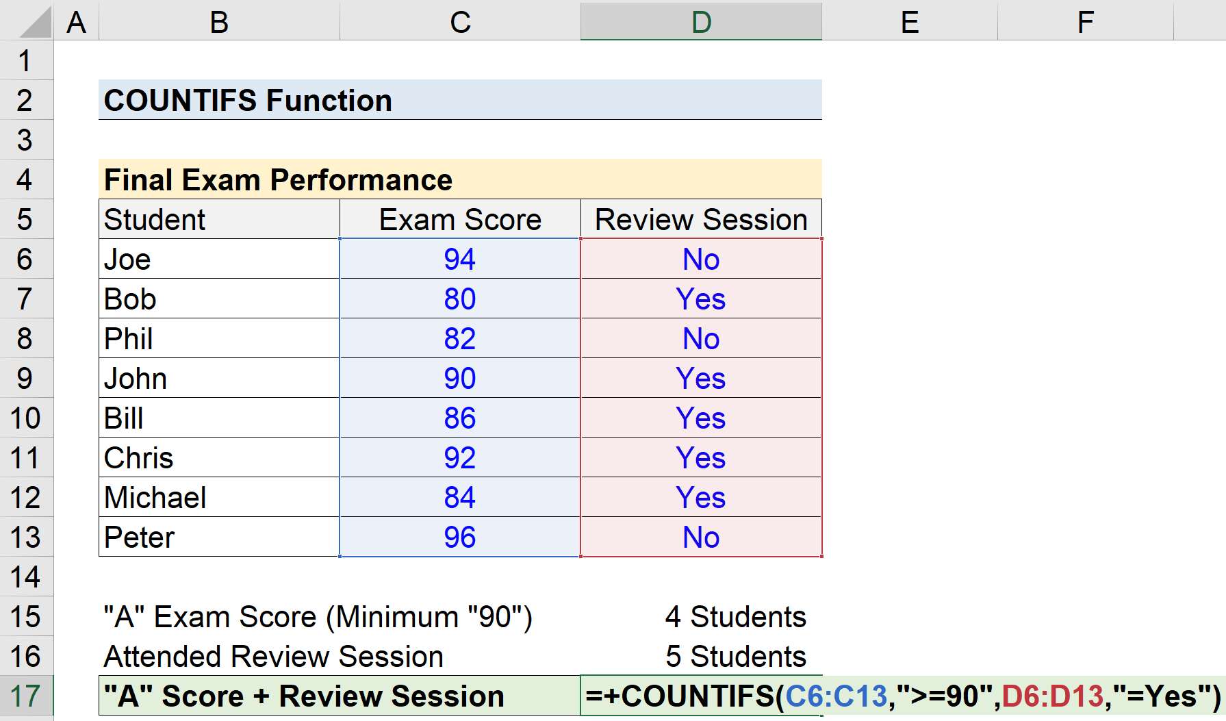
Using the COUNTIFS function, we’ve determined that only two students earned an “A” on the final exam while also having attended the review session.
Therefore, there is insufficient data to conclude that attending the final exam review session was a major determinant in the final exam scores of the students.