Skip to main content
- How to Use XLOOKUP Function in Excel
- What is XLOOKUP Function in Excel?
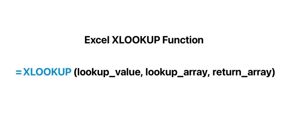
- Excel XLOOKUP Function Formula Syntax
- Excel XLOOKUP Calculator
- 1. XLOOKUP Scenario Analysis Example
- 2. XLOOKUP Return Multiple Values Example
- Excel XLOOKUP Training Tutorial: Complete Walk-Through
- XLOOKUP vs. VLOOKUP: Which is Better?
- XLOOKUP vs. Index Match vs. Offset Match
- Excel XLOOKUP Function: Video Walk-Through
How to Use XLOOKUP Function in Excel
The XLOOKUP Function in Excel searches a dataset in a range or array to return the corresponding value(s) based on user-defined criteria.
What is XLOOKUP Function in Excel?
The XLOOKUP function in Excel was designed as an improvement to existing functions such as the VLOOKUP and HLOOKUP functions, as well as the INDEX/MATCH combination.
The Excel XLOOKUP function enables a user to quickly search for a value in a dataset to return the corresponding value in a different row or column.
The XLOOKUP function was released as part of Office 365 to serve as a more modern, convenient replacement to numerous Excel functions, namely the VLOOKUP function.
The XLOOKUP function can retrieve values vertically or horizontally, and even return entire rows or columns, rather than returning a single value.
The syntax of XLOOKUP is also far more intuitive relative to more outdated Excel functions.
With regard to workflow efficiency, the XLOOKUP function in Excel is more optimal for completing most tasks because of the option to define the “lookup_array” and the “return_array” separately.
Given the user-defined lookup_value, the XLOOKUP function searches for the matching value in the selected lookup_array and then returns the corresponding value (or row) from the selected return_array.
Excel XLOOKUP Function Formula Syntax
The formula syntax for the XLOOKUP function in Excel is as follows.
The XLOOKUP function syntax contains a total of six arguments. Of these, there are three mandatory inputs, whereas the other three are optional inputs that can be omitted.
- lookup_value → The specific value to search for and match
- lookup_array → The array in which the function will search for the matching lookup value
- return_array → The array from which the function will retrieve and return the corresponding value based on the position
- [if_not_found] → The value to return if the lookup value cannot be found – if left omitted, an “N/A” error message is returned
- [match_mode] → The specific type of match necessary here can be described here
- 0: Exact Match (Default)
- -1: Exact Match, Next Smaller Value
- 1: Exact Match, Next Larger Value
- 2: Partial Matching Using Wildcards (“*”,”~”)
- [search_mode] → The order that the XLOOKUP function should abide by while searching the lookup_array
- 1: Top to Bottom, i.e. First Item to Last Item (Default)
- -1: Bottom to Top, i.e. Last Item to First Item
- 2: Binary Search (Ascending Order)
- -2: Binary Search (Descending Order)
Excel XLOOKUP Calculator
We’ll now move to a modeling exercise, which you can access by filling out the form below.
1. XLOOKUP Scenario Analysis Example
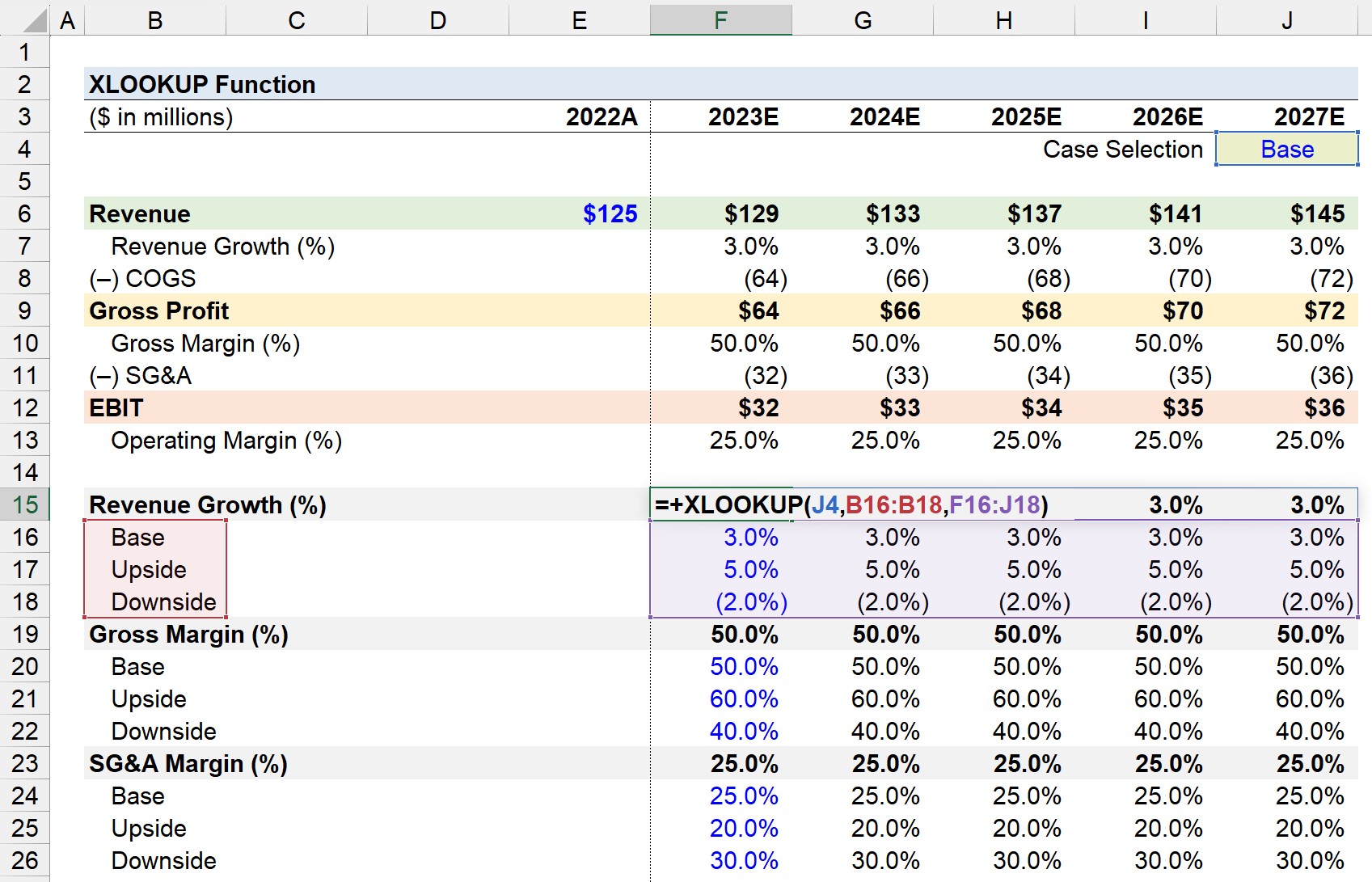
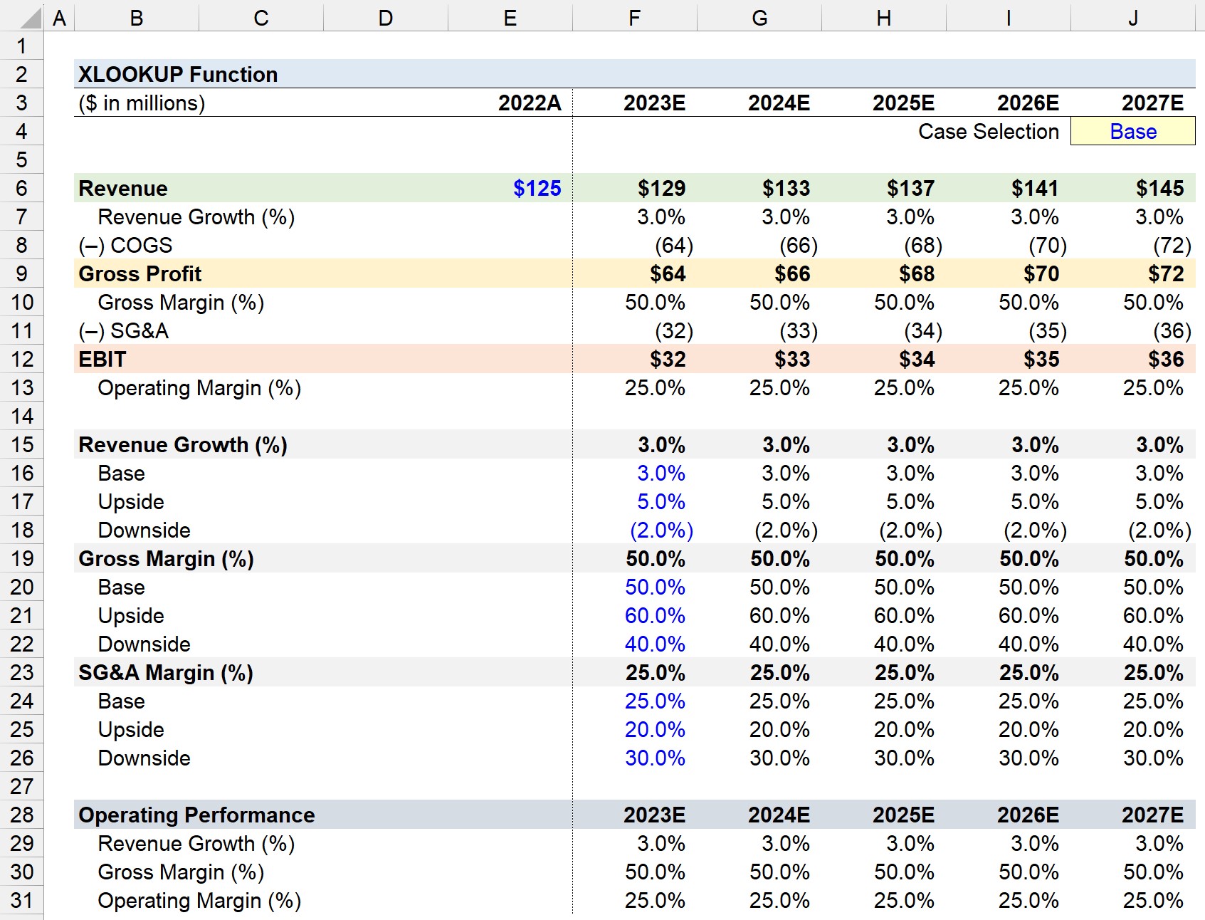
In the first portion of our tutorial on using XLOOKUP in Excel, we’ll use the function to perform scenario analysis as part of creating a five-year forecast model.
There are three operating assumptions in our forward-looking projection model that will determine the pro forma figures. For each operating driver, we’ll set up three cases (e.g. “Base”, “Upside”, and “Downside”), which each reflect a different outcome in terms of operating performance.
- Base = 3.0%
- Upside = 5.0%
- Downside = (2.0%)
Gross Margin (%)
- Base = 50.0%%
- Upside = 60.0%
- Downside = 40.0%
SG&A Margin (%)
- Base = 25.0%
- Upside = 20.0%
- Downside = 30.0%
For the sake of simplicity, the operating assumptions will be straight-lined across the entire forecast, i.e. we will set the cell on the right equal to the cell value on the left.
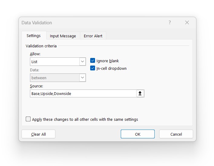
The steps to create a drop-down list in Cell J4 to select the active case are as follows.
- Select the Cell (J4) to Create the Drop-Down List
- Open Data Validation: Press Alt → A → V → V (“Data” → “Data Tools” → “Data Validation”)
- Select “List” as the Criteria from the Settings Tab
- Enter the Cell Values for the Criteria (“Base, Upside, Downside”)
Once the drop-down list is set up, we’ll input our XLOOKUP formula in the operating assumptions section, so that the corresponding assumption is returned based on the active case.
For instance, for the “Revenue Growth (%)” assumption, our formula’s first input is the “Case Selection”. Given the active case, the XLOOKUP function will match the selection to the row containing the exact match. From that point, we’ll select the return array – i.e. the dataset containing the assumptions – and the function will return the coinciding cell value based on the positioning.
Since our model’s case selection is set to “Base”, the XLOOKUP function will return the 3.0% revenue growth rate assumption for each forecast period.
Once we confirm the correct assumptions are being retrieved, we’ll repeat the process for the gross margin and SG&A margin assumptions.
The “COGS” line item is the difference between the gross profit and revenue, while the “SG&A” expense line item equals the SG&A margin multiplied by revenue.
Note: Because COGS and SG&A are each cash outflows, ensure revenue and gross profit are being reduced by these items, i.e. there is a negative sign convention.
2. XLOOKUP Return Multiple Values Example
In the next section of our Excel tutorial, we’ll practice returning multiple values using XLOOKUP by presenting our “Operating Performance” section to summarize the financial results.
Starting with “Revenue Growth (%)”, we’ll select the cell itself, and select the array of rows to search within to identify the match.
By default, the XLOOKUP function in Excel will search from top to bottom since we did not specify the order, i.e. that particular input was omitted (and left blank).
From there, our third selection is the comprehensive data set containing the projected financial data and operating assumptions.
The matching row here is Row 7, so the row of growth rates returned in our operating performance section is 3.0% for the entire forecast period, from 2023E to 2027E.
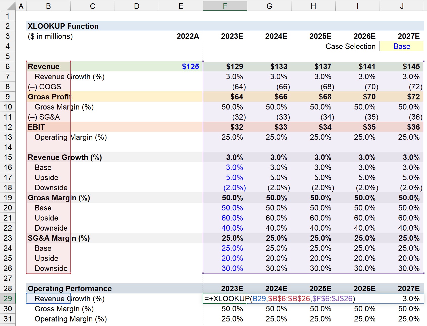
In conclusion, we’ll repeat the same steps for “Gross Margin (%)” and “Operating Margin (%)”. To streamline the process – where the formula can simply be dragged down or copy-pasted – the “lookup_array” and “return_array” should be anchored by pressing the “F4” key once.
Like earlier, the XLOOKUP function in Excel will retrieve and return the cell values that match the initially selected cell and the corresponding values, which are 50.0% and 25.0% for the gross margin and operating margin under the “Base” case, respectively.
Excel XLOOKUP Training Tutorial: Complete Walk-Through
Suppose you’re working with the following employee data set in Excel and tasked with retrieving specific values based on a predefined criteria.

Prior to XLOOKUP, if you wanted to identify Elen Bates’ compensation dynamically – such that a user can select Elen’s last name from a dropdown, you would likely build a VLOOKUP function as follows:

To make the formula work, you’d have to identify the exact column index number – in this case “5” – and you’d have to make sure that the table array starts with the Last Name column.
Of course this made VLOOKUP very brittle – adding columns would always break the formula without additional work to make the formula dynamic:

XLOOKUP vs. VLOOKUP: Which is Better?
XLOOKUP resolves all of this by replacing the table array parameter with 2 new array parameters – the lookup array and the return array. This simple and elegant change makes everything so much less brittle and so much more dynamic:

While the XLOOKUP function has 5 parameters, only the first 3 are required – the lookup value (in our case the Bates last name), the lookup array (in our case the array containing the Bates last name) and the return array (in our case the array containing the compensation data).

We’ll explain the other 2 in a separate post, but the vast majority of use cases only require the first 3.
XLOOKUP vs. Index Match vs. Offset Match
If you have used Excel much in the past, you’re probably familiar with another fix for the problems we just described relating to VLOOKUP and HLOOKUP, namely the index-match combination.
Of course, index match worked great – and continues to work – but in comparison to XLOOKUP now adds more complexity than required. It pains every fiber of my being to retire index-match since it’s done so much heavy lifting for me on the job, but here you can see old reliable offset match doing the same thing XLOOKUP is doing, albeit with a much more complex (and error prone) formula: