Skip to main content
- What is the Excel SUMPRODUCT Function?
- How to Use SUMPRODUCT Function in Excel (Step-by-Step)
- Excel SUMPRODUCT Function Formula Syntax
- SUMPRODUCT Function Calculator — Excel Model Template
- Step 1. SUMPRODUCT Interest Expense Calculation Example
- Step 2. SUMPRODUCT Weighted Average Interest Rate Calculation
What is the Excel SUMPRODUCT Function?
The SUMPRODUCT Function in Excel is a two-fold calculation that first calculates the product of two cells in an array, followed by the sum of those values.
How to Use SUMPRODUCT Function in Excel (Step-by-Step)
The Excel “SUMPRODUCT” function is used to calculate the sum of the products within a given array.
The SUMPRODUCT function is a built-in feature of Excel that combines two commonly used functions.
- “SUM” Function → Adds the values of two or more selected cells to calculate the total.
- “PRODUCT” Function → Multiplies two or more selected values to calculate the product.
For instance, a company might want to calculate the total sales generated on a particular date for a set of products.
Given two columns—the price of the product and the respective quantity sold—the SUMPRODUCT function in Excel can be used to calculate how much in sales was brought in for that specific date.
In Microsoft 365, however, the SUM function in Excel has been updated to become more functional to work with arrays. As a result, entering “SUM” into the spreadsheet and selecting two arrays with a multiplication sign (*) in between will result in the same value as the SUMPRODUCT function.
Excel SUMPRODUCT Function Formula Syntax
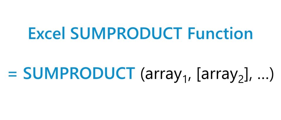
The formula for using the SUMPRODUCT function in Excel is as follows.
- “array1” → The first argument is the array in which the cells are multiplied and then added. A minimum of one array must be selected.
- “array2” → The second array and all the inputs that follow are optional. The total number of arrays that can be entered is capped at 255.
SUMPRODUCT Function Calculator — Excel Model Template
We’ll now move on to a modeling exercise, which you can access by filling out the form below.
Step 1. SUMPRODUCT Interest Expense Calculation Example
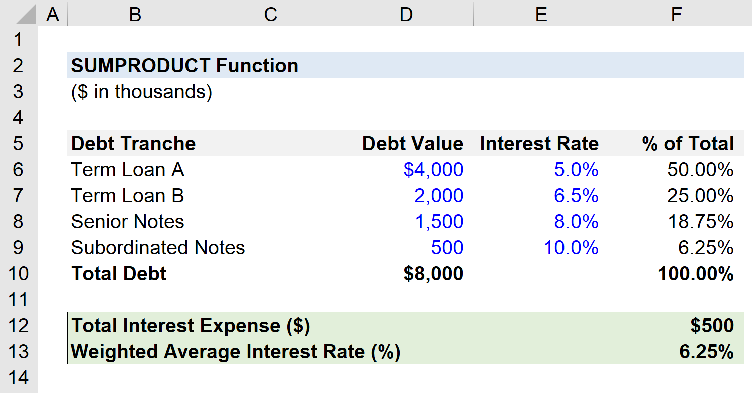
Suppose we’re tasked with calculating the total interest expense owed by a company.
The left column contains the debt tranche, while the two columns on the right state the corresponding debt value ($) and the specific interest rate (%) attached to each tranche.
The fourth column calculates the total percentage contribution of the given debt tranche to the total debt outstanding.
There are four types of debt on the company’s balance sheet, and for the sake of simplicity, we’ll assume a fixed interest rate on each tranche.
| Debt Tranche | Debt Value ($) | Interest Rate (%) | % of Total |
|---|---|---|---|
| Term Loan A (TLA) | $4,000,000 | 5.0% | 50.0% |
| Term Loan B (TLB) | $2,000,000 | 6.5% | 25.0% |
| Senior Notes | $1,500,000 | 8.0% | 18.8% |
| Subordinated Notes | $500,000 | 10.0% | 6.3% |
Using the SUMPRODUCT function in Excel, we’ll first calculate the total interest expense obligation of the company.
The arrays that we’ll select are the debt values and the interest rates.
The formula that we enter into Excel is as follows.
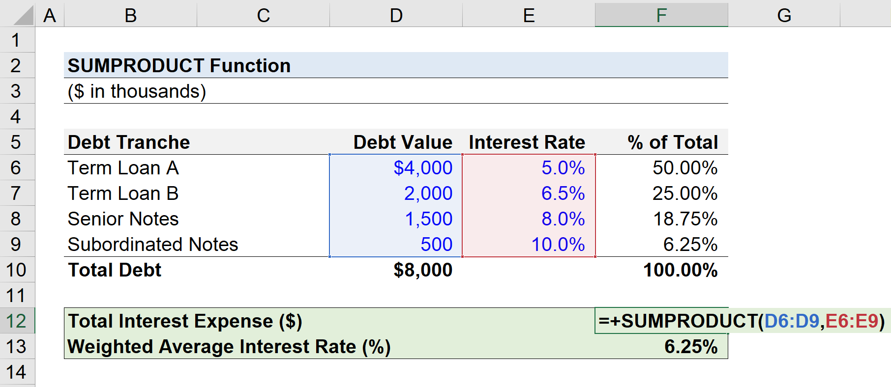
The interest expense owed on the $8 million in debt obligations, assuming our hypothetical scenario is on an annual basis, is implied to be $500,000.
- Total Interest Expense = $500,000
Step 2. SUMPRODUCT Weighted Average Interest Rate Calculation
In the next part of our Excel tutorial, we’ll calculate the weighted average interest rate using the same data set as earlier.
The weighted average interest rate of a company’s debt can be a useful approximation for the company’s overall cost of debt, albeit it is still meant to be an estimate.
Earlier, we were already provided with the percentage contribution of each debt tranche, which is equal to the debt value divided by the total debt balance.
Thus, the only remaining step is to use the SUMPRODUCT function, where the selected arrays are the interest rates (%) and the percentage contribution (%).
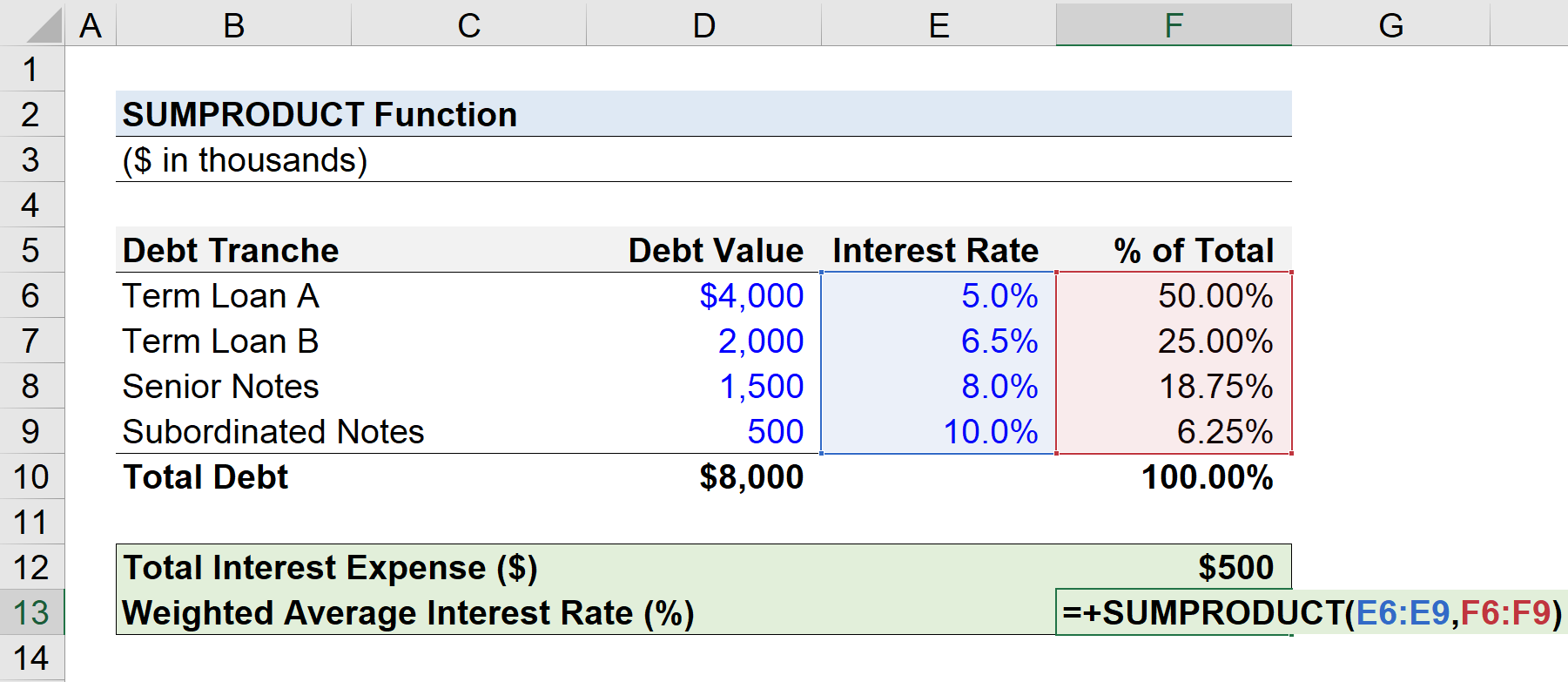
In closing, the weighted average interest rate is 6.25%.
- Weighted Average Interest Rate (%) = 6.25%