- What is Discount Rate?
- How to Calculate Discount Rate
- Discount Rate Formula
- Discount Rate vs. NPV: What is the Difference?
- Why is the Discount Rate Important?
- Refining Discount Rate Selection Through AI
- WACC vs. Cost of Equity: What is the Difference?
- Full-Form Discount Rate: What are the Components?
- Discount Rate Calculator
- 1. Cost of Debt Calculation Example (kd)
- 2. Cost of Equity Calculation Example (ke)
- 3. Capital Structure Analysis Example
- 4. Discount Rate Calculation Example
What is Discount Rate?
The Discount Rate is the minimum rate of return expected to be earned on an investment given its risk profile. The present value (PV) of the future cash flows generated by a company is estimated using an appropriate discount rate – i.e. the opportunity cost of capital – which reflects the riskiness of the underlying company (or investment).
How to Calculate Discount Rate
The discount rate, often called the “cost of capital”, is the minimum rate of return necessary to invest in a particular project or investment opportunity.
In corporate finance, the discount rate reflects the necessary return on an investment, such as common stock, given the riskiness of its future cash flows.
Conceptually, the discount rate estimates the risk and potential returns of an investment – therefore, a higher rate implies greater risk but also more upside potential.
In part, the estimated discount rate is determined by the time value of money (TVM) – i.e. a dollar today is worth more than a dollar received on a future date – and the return on comparable investments with similar risks.
Interest can be earned over time if the capital is received on the current date. Hence, the discount rate is often referred to as the opportunity cost of capital, and functions as the hurdle rate to guide decision-making around capital allocation and selecting worthwhile investments.
When considering an investment, the rate of return that an investor should reasonably expect to earn depends on the returns on comparable investments with similar risk profiles.
The discount rate can be calculated using the following three-step process:
- First, the value of a future cash flow (FV) is divided by the present value (PV)
- Next, the resulting amount from the prior step is raised to the reciprocal of the number of years (n)
- Finally, one is subtracted from the value to calculate the discount rate
Discount Rate Formula
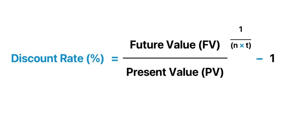
The discount rate formula divides the future value (FV) of a cash flow by its present value (PV), raises the result to the reciprocal of the number of periods, and subtracts by one.
For instance, suppose your investment portfolio has grown from $10,000 to $16,000 across a four-year holding period.
- Future Value (FV) = $16,000
- Present Value (PV) = $10,000
- Number of Periods = 4 Years
If we plug those assumptions into the formula from earlier, the discount rate is approximately 12.5%.
- Discount Rate (r) = ($16,000 ÷ $10,000) ^ (1 ÷ 4) – 1 = 12.47%
The example we just completed assumes annual compounding, i.e. 1x per year.
However, rather than annual compounding, if we assume that the compounding frequency is semi-annual (2x per year), we would multiply the number of periods by the compounding frequency.
Upon adjusting for the effects of compounding, the discount rate comes out to be 6.05% per 6-month period.
- Discount Rate (r) = ($16,000 ÷ $10,000) ^ (1 ÷ 8) – 1 = 6.05%
Discount Rate vs. NPV: What is the Difference?
The net present value (NPV) of a future cash flow equals the cash flow amount discounted to the present date.
With that said, a higher discount rate reduces the present value (PV) of future cash flows (and vice versa).
In the formula above, “n” is the year when the cash flow is received. The further the cash flow is received, the greater the reduction.
Moreover, a fundamental concept in valuation is that incremental risk should coincide with greater return potential.
- Higher Discount Rate → Lower Net Present (NPV)
- Lower Discount Rate → Higher Net Present Value (NPV)
Therefore, the expected return is set higher to compensate the investors for undertaking the risk.
If the expected return is insufficient, it would not be reasonable to invest, as there are other investments elsewhere with a better risk/return trade-off.
On the other hand, a lower discount rate causes the valuation to rise, because such cash flows are more certain to be received.
More specifically, future cash flows are more stable and likely to occur in the foreseeable future. Therefore, stable, market-leading companies like Amazon and Apple tend to exhibit lower discount rates.
Learn More → Discount Rate by Industry (Damodaran)
Why is the Discount Rate Important?
In a discounted cash flow analysis (DCF), the intrinsic value of an investment is based on the projected cash flows generated, which are discounted to their present value (PV) using the discount rate.
Once all the cash flows are discounted to the present date, the sum of all the discounted future cash flows represents the implied intrinsic value of an investment, most often a public company.
The discount rate is a critical input in the DCF model – in fact, the discount rate is arguably the most influential factor to the DCF-derived value.
One rule to abide by is that the discount rate and represented stakeholders must align.
The appropriate discount rate to use is contingent on the represented stakeholders:
- Weighted Average Cost of Capital (WACC) → All Stakeholders (Debt + Equity)
- Cost of Equity (ke) → Common Shareholders
- Cost of Debt (kd) → Debt Lenders
- Cost of Preferred Stock (kp) → Preferred Stock Holders

Refining Discount Rate Selection Through AI
Selecting an accurate discount rate is vital for precise valuations, but it often depends on subjective estimates that can lead to inconsistencies. Artificial intelligence enhances this process by analyzing vast datasets, including historical market trends, comparable company metrics, and macroeconomic indicators. Finance professionals can make data-driven decisions when choosing a discount rate by applying skills taught in the AI for Business & Finance Certificate Program, a collaboration between Wall Street Prep and Columbia Business School Executive Education that equips participants with advanced AI forecasting tools.
WACC vs. Cost of Equity: What is the Difference?
- WACC → FCFF: The weighted average cost of capital (WACC) reflects the required rate of return on investment for all capital providers, i.e. debt and equity holders. Since both debt and equity providers are represented in WACC, the free cash flow to firm (FCFF) – which belongs to both debt and equity capital providers – is discounted using the WACC.
- Cost of Equity → FCFE: In contrast, the cost of equity is the minimum rate of return from the viewpoint of only equity shareholders. The free cash flow to equity (FCFE) belonging to a company should be discounted using the cost of equity, as the represented capital provider in such a case is common shareholders.
Thereby, an unlevered DCF projects a company’s FCFF, which is discounted by WACC – whereas a levered DCF forecasts a company’s FCFE and uses the cost of equity as the discount rate.
Full-Form Discount Rate: What are the Components?
The weighted average cost of capital (WACC) represents the opportunity cost of an investment based on comparable investments of similar risk profiles.
Formulaically, the WACC is calculated by multiplying the equity weight by the cost of equity and adding it to the debt weight multiplied by the tax-affected cost of debt.
Where:
- E / (D + E) = Equity Weight (%)
- D / (D + E) = Debt Weight (%)
- ke = Cost of Equity
- kd = After-Tax Cost of Debt
Unlike the cost of equity, the cost of debt must be tax-effected, because interest expense is tax-deductible, i.e. the interest “tax shield.”
To tax affect the pre-tax cost of debt, the rate must be multiplied by one minus the tax rate.
The capital asset pricing model (CAPM) is the standard method used to calculate the cost of equity.
Based on the CAPM, the expected return on a security is a function of the issuer’s sensitivity to the broader market, typically approximated as the returns of the S&P 500 index.
There are three components in the CAPM formula:
| CAPM Components | Description |
|---|---|
| Risk Free Rate (rf) |
|
| Equity Risk Premium (ERP) |
|
| Beta (β) |
|
Calculating the cost of debt (kd), unlike the cost of equity, tends to be relatively straightforward because debt issuances like bank loans and corporate bonds have readily observable interest rates via sources such as Bloomberg.
Conceptually, the cost of debt is the minimum return that debt holders demand before bearing the burden of lending debt capital to a specific borrower.
Discount Rate Calculator
We’ll now move to a modeling exercise, which you can access by filling out the form below.
1. Cost of Debt Calculation Example (kd)
Suppose we’re tasked with calculating the weighted average cost of capital (WACC) for a company.
Our first step is to compute the cost of debt.
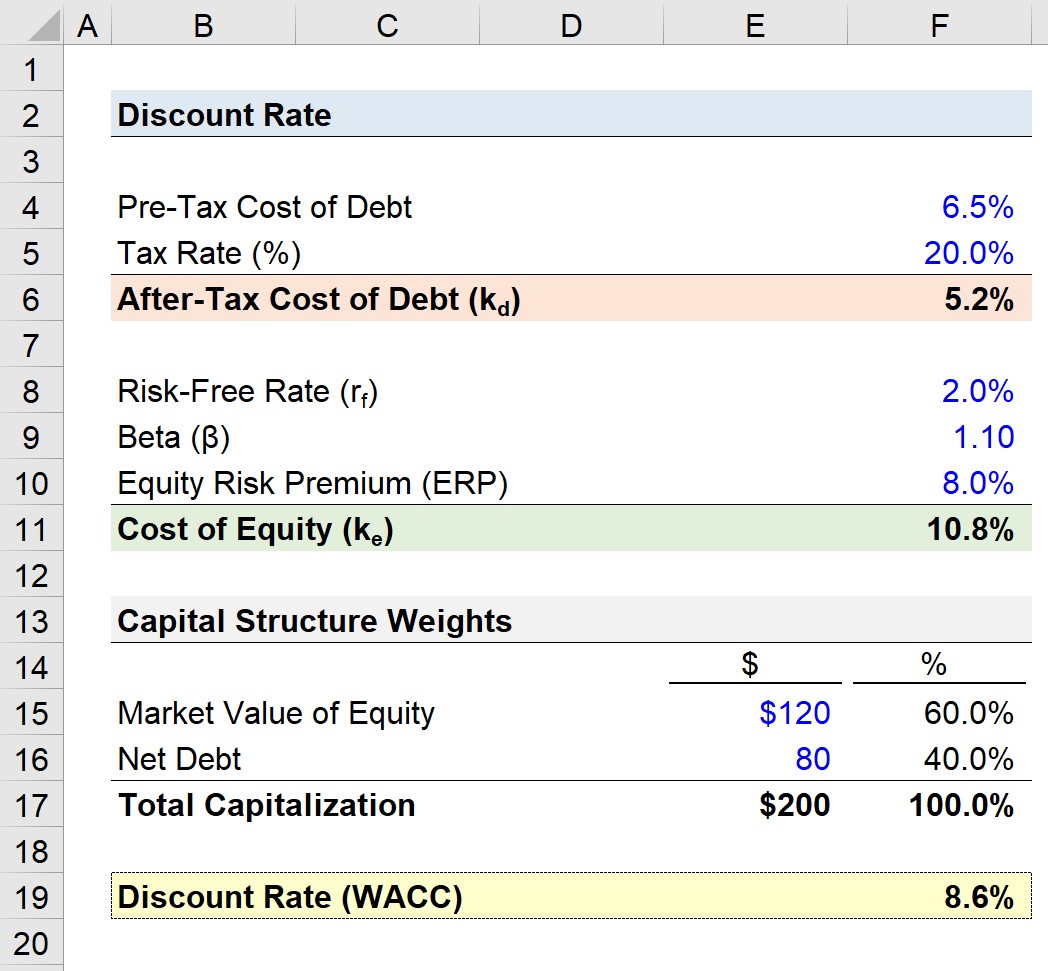
If we assume the company has a pre-tax debt cost of 6.5% and the tax rate is 20.0%, the after-tax debt cost is 5.2%.
- After-Tax Cost of Debt (kd) = 6.5% × (1 – 20.0%)
- kd = 5.2%
2. Cost of Equity Calculation Example (ke)
The next step is to calculate the cost of equity using the capital asset pricing model (CAPM).
The three assumptions for our three inputs are as follows:
- Risk-Free Rate (rf) = 2.0%
- Beta (β) = 1.10
- Equity Risk Premium (ERP) = 8.0%
If we enter those figures into the CAPM formula, the cost of equity comes out to 10.8%.
- Cost of Equity (ke) = 2.0% + (1.10 × 8.0%)
- ke = 10.8%
3. Capital Structure Analysis Example
We must now determine the capital structure weights, i.e. the % contribution of each source of capital.
The market value of equity – i.e. the market capitalization (or equity value) – is assumed to be $120 million. On the other hand, the net debt balance of a company is assumed to be $80 million.
- Market Value of Equity = $120 million
- Net Debt = $80 million
While the market value of debt should be used, the book value of debt shown on the balance sheet is usually fairly close to the market value (and can be used as a proxy should the market value of debt not be available).
The intuition behind the use of net debt is that cash on the balance sheet could hypothetically be used to pay down a portion of the outstanding gross debt balance.
By adding the $120 million in equity value and $80 million in net debt, we calculate that the total capitalization of our company equals $200 million.
From that $200 million, we can determine the relative weights of debt and equity in the company’s capital structure:
- Equity Weight = 60.0%
- Debt Weight = 40.0%
4. Discount Rate Calculation Example
We now have the necessary inputs to calculate our company’s discount rate, which is equal to the sum of each capital source cost multiplied by the corresponding capital structure weight.
- Discount Rate (WACC) = (5.2% × 40.0%) + (10.8% × 60.0%)
- WACC = 8.6%
In closing, the discount rate (or cost of capital) of our hypothetical company comes out to 8.6%, which is the implied rate used to discount its future cash flows.
Everything You Need To Master Financial Modeling
Enroll in The Premium Package: Learn Financial Statement Modeling, DCF, M&A, LBO and Comps. The same training program used at top investment banks.
Enroll Today
")