 Skip to main content
- What is Bottom Up Forecasting?
- How to Perform Bottom Up Forecasting
- Bottom-Up vs. Top-Down Forecasting: What is the Difference?
- Bottom Up Forecasting Formula
- Core Revenue Drivers: Unit Economics by Industry
- Bottom Up Forecasting Calculator
- 1. Revenue Forecast Model Operating Assumptions
- 2. Revenue Forecasting Assumptions with Operating Cases
- 3. Bottom-Up Revenue Build
- 4. Net Revenue Forecast Example
- 5. Bottom-Up Forecasting Calculation Example
What is Bottom Up Forecasting?
Bottom Up Forecasting consists of breaking a business apart into the underlying components that ultimately drive its revenue generation, profits, and growth.

How to Perform Bottom Up Forecasting
The bottom-up forecasting method relies on granular, product-level historical financial and operating data, including the insights derived from analyzing current market trends and comparables.
Each bottom-up forecast model differs based on the specific unit economics that impacts the financial performance of a given company.
Yet, for all companies, a detailed forecast is imperative for properly establishing goals, budgeting and setting revenue targets for all companies.
The fundamentals-oriented approach is thereby viewed as more logical because the thought process behind each assumption can be supported and explained in detail.
Using the insights derived from a robust bottom-up forecast, the management team of a company can more accurately anticipate revenue in real-time as new data on customer demand and monthly sales come in, as well as predict fluctuations such as cyclicality or seasonality.
If the actual anticipated financial results of a company end up deviating from initial projections, the company can then assess and understand the reasoning behind why the actual results were below (or exceeded) expectations in order for the proper adjustments to be made.
Bottom-Up vs. Top-Down Forecasting: What is the Difference?
The purpose of a bottom-up forecast should be to output informative data that leads to decision-making supported by tangible data.
Bottom-up projection models enable management teams to develop a better perception of their business, which precedes improved operational decision-making.
Compared to the top-down forecasting approach, the bottoms-up forecast is much more time-consuming, and sometimes, can become even too granular.
The key is being granular enough that assumptions can easily be supported by historical financial data and other supportable findings, but not so granular that the construction and maintenance of the forecast is unsustainable.
If a financial model is composed of too many different data points, the model can become inflexible and overly complex (i.e., “less is more”).
For any model to be useful, the level of detail must be properly balanced with the right drivers of revenue identified to effectively serve as the core infrastructure of the model.
Otherwise, the risk of becoming lost in the details is too substantial, which defeats the benefits of forecasting in the first place.
Another potential drawback is that the approach increases the probability of receiving scrutiny from outside parties like investors.
While a top-down forecast is broadly oriented around a prediction that the company can capture a certain market share percentage, a bottoms-up forecast leads to setting specific goals and opens up the door for more criticism.
This is inevitable as specificity when setting financial targets tends to be interpreted by stakeholders (or the public) as being more precise – and thus, held to a higher standard with regards to accuracy.
But in general, a bottoms-up forecast is viewed as being far more versatile, as well as more meaningful in terms of how valuable the model-derived insights are.
Bottom Up Forecasting Formula
Unlike top-down forecasts, bottom-up forecasts can be driven off an extensive variety of industry-specific assumptions.
However, at its core, all bottom-up models essentially follow the same base formula:
The Wharton Online & Wall Street Prep Applied Value Investing Certificate Program
Learn how institutional investors identify high-potential undervalued stocks. Enrollment is open for the upcoming cohort.
Enroll TodayCore Revenue Drivers: Unit Economics by Industry
The unit economics used is going to be company-specific, but common examples of metrics used to calculate revenue include:
| Industry | Price Metrics | Quantity Metrics |
| B2B Software |
|
|
| Online B2C / D2C Businesses |
|
|
| E-Commerce Platforms (or Marketplace) |
|
|
| In-Person Stores (e.g., Retail) |
|
|
| Trucking Transportation (Freight / Distribution) |
|
|
| Airline Industry |
|
|
| Sales-Oriented Companies (e.g., Enterprise Software Sales, M&A Advisory) |
|
|
| Healthcare Sector (e.g., Hospitals, Medical Clinics) |
|
|
| Hospitality Industry |
|
|
| Subscription-Based Companies (e.g., Streaming Networks) |
|
|
| Social Media Networking Companies (Advertising-Based) |
|
|
| Services-Based Companies (e.g., Consulting) |
|
|
| Financial Institutions (Banks) |
|
|
The process of selecting the right metrics to use is similar to that of picking the variables for a sensitivity analysis, in which the practitioner must choose relevant variables that have a material impact on the financial performance of the company (or the returns).
Bottom Up Forecasting Calculator
We’ll now move on to a modeling exercise, which you can access by filling out the form below.
1. Revenue Forecast Model Operating Assumptions
In our example tutorial, the hypothetical scenario used in our bottoms-up forecast is of a direct-to-consumer (“D2C”) company with roughly $60mm in LTM revenue.
The D2C company sells a single product with an ASP ranging around $100-$105 in the trailing three years and a low product count per order (i.e., ~1 to 2 products each order historically).
Additionally, the D2C company is considered to be in the late-stage of its developmental lifecycle, as indicated by its sub-20% YoY revenue growth.
We begin by identifying the fundamental drivers of revenue for a standard D2C business:
- Total Number of Orders
- Average Order Value (AOV)
- Average Number of Products Per Order
- Average Selling Price (ASP)
Since we are given the total revenue and the total number of orders for the past three years, we can back out of the estimated average order value (AOV) by dividing the two metrics.
For instance, the AOV in 2018 was $160 and this figure grows to approximately $211 by 2020. Note that we are intentionally using the total revenue as opposed to the net revenue, as we do not want the typical order value to be skewed by refunds.
Later on, we will forecast the refund amounts separately. The inclusion of the refund amount in our formula by using net revenue would cause us to make the mistake of double-counting.
Using the provided “Average Number of Products Per Order”, we can then estimate the ASP for each year by:
The ASP of an individual product comes out to about $100 in 2018, which grows to around $105 in 2020.
2. Revenue Forecasting Assumptions with Operating Cases
Now, we can create assumptions for these drivers with three different scenarios (i.e., Base Case, Upside Case, and Downside Case).
The three variables that we will project are:
- Total Number of Orders % Growth
- Number of Products Per Order % Growth
- Change in Average Selling Price (ASP)
The finished assumption section is shown below.
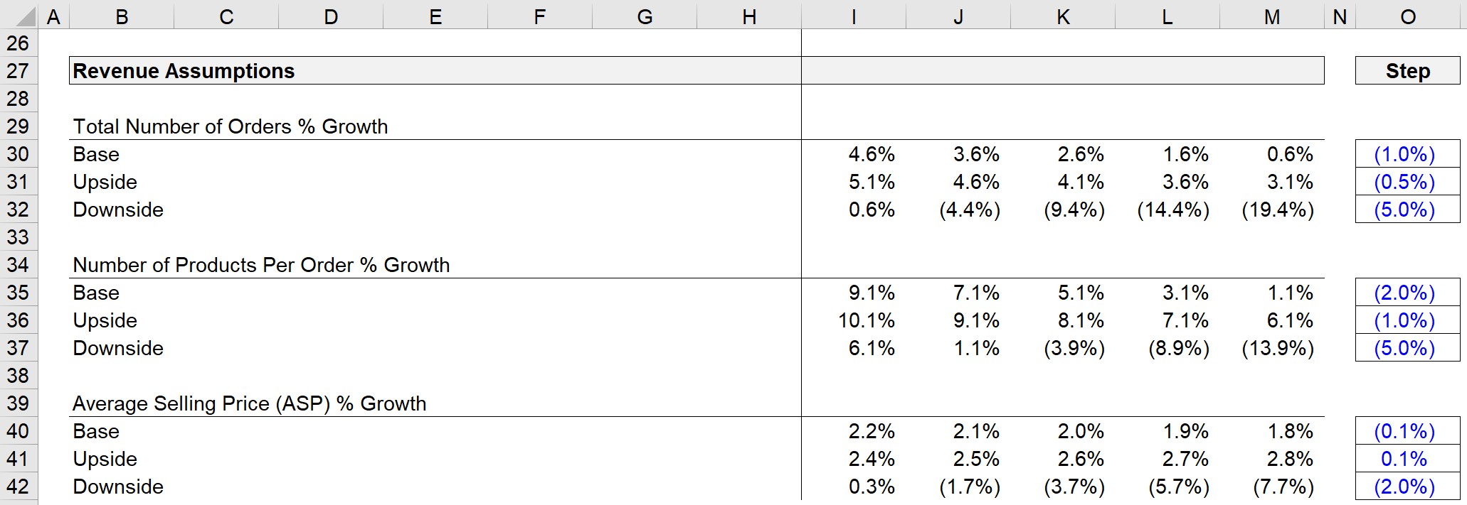
In practice, the assumptions used should take into account:
- Historical Growth Rates
- Comparable Companies’ Forecasts and Pricing Data
- Industry Trends (Tailwinds and Headwinds)
- Competitive Landscape
- Industry Research Reports from 3rd Party Sources
- Estimated Market Sizing (i.e., Sanity Check Assumptions)
With the historical AOVs and ASPs calculated and the forecast of the three drivers ready, we are now prepared for the next step.
3. Bottom-Up Revenue Build
Since we worked our way down to ASP, we will now work our way back up by starting with forecasting ASP.
Here, we will use the XLOOKUP function in Excel to grab the right growth rate based on the active case selection.
The XLOOKUP formula contains three parts, with each pertaining to three distinct scenarios:
- Active Case (e.g., Base, Upside, Downside)
- ASP Array for the 3 Cases – Finds the Line w/ the Active Case
- Array for the ASP Growth Rate – Matched to the Active Case Cell (and Outputs Value)
Therefore, the ASP growth rate for 2021 is 2.2% as the active case is switched to the base case.
Then, the prior year ASP will be multiplied by (1 + growth rate) to arrive at the current year ASP, which comes out to $107.60.
The same XLOOKUP process will be done for the number of products per order.
Note: Alternatively, we could have used the OFFSET / MATCH function.
In 2020, the average number of products per order was 2.0, and after growing by 9.1% YoY, the number of products per order is now ~2.2 in 2021.
The AOV was excluded from the revenue assumptions section, as this metric will be calculated by:
Based on this calculation, the projected AOV in 2021 is about $235 (i.e. ASP is $107.60 and each order contains about 2.2 products on average).
To wrap up the revenue projection assumption linkages, we now grow the total number of orders using XLOOKUP again.
And finally, we can forecast total revenue by using the following formula:
Now, we have all the calculations set for the first projection year, which we can now extrapolate forward for the rest of the forecast.
4. Net Revenue Forecast Example
Returning to refunds, which are very common and must be included in models for e-commerce and D2C companies, we simply divide the historical refund amounts by the total revenue.
The refund as a percentage of total revenue comes out to roughly 0.1%-0.2%. As this is an insignificant number, refunds will be straight-lined. The projected refund amount will be:
With the refund forecast filled out, we can move on to calculating net revenue, which accounts for the refunds and avoids double-counting.
5. Bottom-Up Forecasting Calculation Example
From a glance at our completed bottom-up forecast model, the increase in average order value (AOV) seems to be the primary driver of revenue growth, as seen from the expansion of AOV from $211 in 2020 to $298 by the end of 2025.
However, upon closer look into the same time frame, that 7.2% CAGR of AOV is being driven by the:
- Average Number of Products Per Order: 2.0 → 2.6
- Average Selling Price (ASP): $105 → $116
In closing, we can see that the net revenue of the D2C business is anticipated to grow at a 5-year CAGR of approximately 10% throughout the forecast period.


Do you have an example of this for B2B SaaS? Instead of working up from ASP, would you work up from ACV?
Hi, Samaria,
That’s correct, you would work up from either ACV or average revenue per account (ARPA), rather than ASP, as in B2C business products.
BB