
- What is Security Market Line?
- How Does the Security Market Line (SML) Work?
- Security Market Line Formula (SML)
- Security Market Line Graph Example (SML)
- What is the Slope of the Security Market Line?
- How to Interpret the Slope of SML Graph?
- How to Analyze the Efficient Frontier and Market Equilibrium
- Security Market Line (SML) vs. Capital Market Line (CML): What is the Difference?
What is Security Market Line?
The Security Market Line (SML) is a graphical representation of the capital asset pricing model (CAPM), which reflects the linear relationship between a security’s expected return and beta, i.e. its systematic risk.
How Does the Security Market Line (SML) Work?
In corporate finance, the security market line (SML) visually illustrates the capital asset pricing model (CAPM), one of the fundamental methodologies taught in academia and used in practice to determine the relationship between the expected return on a security given the coinciding market risk.
While the chance of encountering the security market line on the job is practically zero, the capital asset pricing model (CAPM) — from which the SML is derived — is commonly utilized by practitioners to estimate the cost of equity (ke).
The cost of equity (ke) represents the minimum required rate of return expected to be received by common shareholders given the risk profile of the underlying security.
The required rate of return, or “discount rate”, is one of the primary determinants that guide the decision-making process of an investor on whether to invest in the security.
Security Market Line Formula (SML)
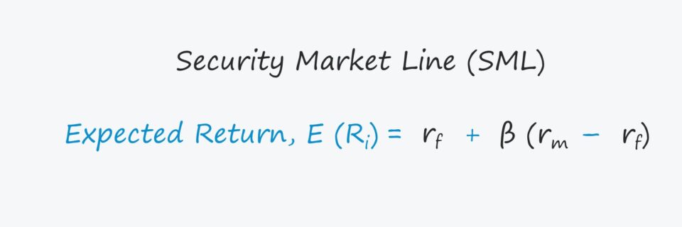
There are three components to the CAPM formula, which are the risk-free rate (rf), the beta (β) and the equity risk premium (ERP).
- Risk Free Rate (rf) → The yield received on risk-free securities, which is most often the 10-year treasury bond issued by the government for companies based in the U.S.
- Beta (β) → The non-diversifiable risk resulting from market volatility (i.e. the systematic risk) of a security relative to the broader market (S&P 500).
- Equity Risk Premium (ERP) → The difference between the expected market return (S&P 500) and the risk-free rate, i.e. the excess return received from investing in public equities over the risk-free rate.
The CAPM equation starts with the risk-free rate (rf), which is subsequently added to the product of the security’s beta and the equity risk premium (ERP) in order to calculate the implied expected return on the investment.
The equity risk premium (ERP) is often used interchangeably with the term “market risk premium” and is calculated by subtracting the risk free rate (rf) from the market return.
The Wharton Online & Wall Street Prep Applied Value Investing Certificate Program
Learn how institutional investors identify high-potential undervalued stocks. Enrollment is open for the upcoming cohort.
Enroll TodaySecurity Market Line Graph Example (SML)
One of the core assumptions inherent to the CAPM equation (and thus, the security market line) is that the relationship between expected return on a security and beta, i.e. the systematic risk, is linear.
The premise of the security market line (SML) is that the expected return of a security is a function of its systematic, or market, risk.
In effect, the SML displays the expected return on an individual security at different levels of systematic risk.
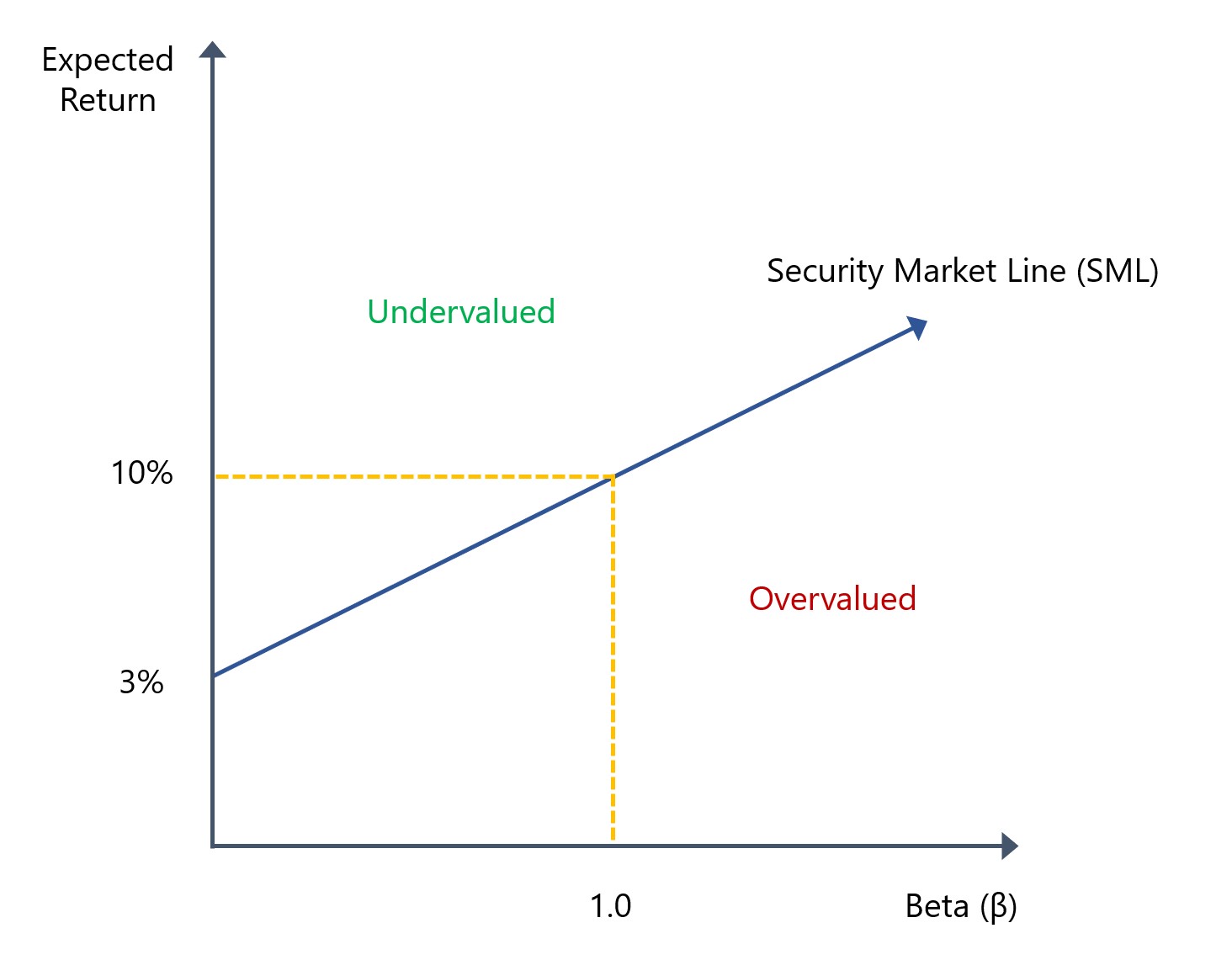
- X-Axis → Beta (β)
- Y-Axis → Expected Return
- Y-Intercept → Risk-Free Rate (rf)
The x-axis represents the systematic risk while the y-axis is the expected rate of return on the security, so the excess return over the expected market return reflects the equity risk premium (ERP).
In our illustrative graph depicting the security market line (SML), the risk free rate is assumed to be 3% and the market return is 10%. Because the beta of the market is 1.0, we can confirm that the expected return comes out to 10%.
Generally speaking, the return on the market (S&P 500) has historically been around ~10% while the equity risk premium (ERP) normally ranges between 5% to 8%.
The point on the y-axis where the SML begins, as one would reasonably assume, is the risk free return (rf). Hence, the SML curve is upward sloping, as the risk free rate (rf) is the minimum yield.
The upward-sloping shape of the curve is because securities with higher systematic risk coincide with a higher expected return from investors, i.e. more risk = more reward.
What is the Slope of the Security Market Line?
The slope of the security market line (SML) is the reward-to-risk ratio, which equals the difference between the expected market return and risk-free rate (rf) divided by the beta of the market.
Since the beta of the market is constant at 1.0, the slope can be re-written as the market return net of the risk free rate, i.e. the equity risk premium (ERP) formula from earlier.
- Slope of SML → Equity Risk Premium (ERP)
Thus, the equity risk premium (ERP) represents the slope of the security market line (SML) and the reward earned by the investor for bearing the stated systematic risk.
The risk premium is meant to compensate the investor for the incremental systematic risk undertaken as part of investing in the security. But if a security is correctly priced by the market, the risk/return profile remains constant and would be positioned on top of the SML.
How to Interpret the Slope of SML Graph?
Fundamentally, a higher degree of systematic risk (i.e. undiversifiable, market risk) in a security should result in investors requiring a higher rate of return as compensation for the greater level of risk.
The placement of the security relative to the security market line determines whether it is undervalued, valued fairly, or overvalued.
- Positioned Above SML → “Undervalued”
- Positioned Under SML → “Overvalued”
Therefore, a security positioned above the SML should exhibit higher returns and lower risk, whereas a security positioned below the SML should expect lower returns in spite of the higher risk.
Intuitively, if the security is above the SML, the expectation is a higher return for the level of risk, albeit the opportunity might’ve been capitalized on by other market participants.
On the other hand, if the security is below the SML, it would be deemed overvalued since lower returns are anticipated while still being exposed to a greater level of risk.
How to Analyze the Efficient Frontier and Market Equilibrium
The efficient frontier is the set of optimal positions where the expected return is maximized given the set risk level, i.e. the target risk/return trade-off is reached.
In theory, the market has correctly priced the security if it can be plotted directly on the SML, i.e. the market is in a state of “perfect equilibrium”.
In a state of market equilibrium, the asset in question possesses the same reward-to-risk profile as the broader market.
The securities that lie below the efficient frontier provide inadequate returns given the pre-defined level of risk, with the reverse being true for securities above and to the right, wherein there is excessive risk for the anticipated return.
Security Market Line (SML) vs. Capital Market Line (CML): What is the Difference?
The security market line (SML) is frequently mentioned alongside the capital market line (CML), but there are notable differences to be aware of:
- Security Market Line (SML) → Risk/Return Trade-Off for Individual Securities
- Capital Market Line (CML) → Risk/Return Trade-Off for a Portfolio
While both illustrate the relationship between risk and the expected return with similar rules for interpreting the position (i.e. above line = underpriced, plot on the line = fairly priced and below line = overpriced), one key distinction is the measure of risk.
In the capital market line (CML), the risk measure is the standard deviation of the portfolio returns rather than beta, as is in the case of the SML.
The Wharton Online & Wall Street Prep Applied Value Investing Certificate Program
Learn how institutional investors identify high-potential undervalued stocks. Enrollment is open for the upcoming cohort.
Enroll Today


